Creating a Flag using Bezier Surfaces

In this post, I will explain my experience with the first assignment of CENG 469 Computer Graphics 2 course, in which we are asked to implement a waving flag with Bezier surfaces.

Devlog Video

I was recording a devlog while doing the project. However, as the deadline closed in, I focused on the project and couldn’t finish the devlog.

Here’s the incomplete devlog, starts off serious but goes downhill from there:

The video tells more about the initial stages of the project.

Getting Started

Thanks to our professors and teaching assistants, we were given a sample OpenGL program to get started. This program handles all of the essential functions of a basic OpenGL program, such as creating a window, reading and compiling shaders, etc. It also features more advanced stuff, e.g., an .obj parser.

I started by removing the unnecessary parts. Since we will generate all the geometry in run-time in this assignment, I removed the .obj parser. Then, I removed the custom struct definitions and opted to use the alternatives presented in glm library. glm library is comprehensive, and it can handle all fundamental linear algebra operations. Therefore, I didn’t want to reinvent the wheel.

Bezier Surface

Implementing a bezier surface was much easier than I thought. Essentially, all you have to do is

1. Create 3 4x4 matrices for x, y, and z. These matrices will hold the positions of the control points. We will call these matrices \(Z\), or use \(Z_x\), \(Z_y\), \(Z_z\) to refer to particular one.
2. Create the constant \(M_B\) basis matrix.
   • I ran into a problem during this step: glm stored the matrices in column-wise order. Consequently, if you write the values in the matrix as you see them into a glm::mat4, you will actually get the transpose of that matrix.
3. Given \(s\) and \(t\) parameters, compute \(S = [s^3, s^2, s, 1]\) and \(T = [t^3, t^2, t, 1]\).
4. Find the point \(Q(s,t)\) by calculating \(S M_B Z M_B^T T^T\) for all \(Z\).

In the slides, there’s an alternate method without using matrices, but I think that it’s actually harder to implement and it might yield worse performance. Since the matrix operations are extremely common, the library developers do their best to optimize them.

At this point, I had a basic program that can display a flat Bezier surface. I’m skipping the screenshots for now since it’s not interesting.

Adding Texture

Adding a texture was easy. The assignment document recommended to use stb_image.h header-only library for reading the images. In the prerequisite computer graphics course CENG 477, we used another library, albeit the code was much longer and verbose, hence harder to read. Because of these reasons, I liked this library a lot and I will definitely prefer it in the future if it’s adequate for my purposes.

I was already familiar with handling the textures with OpenGL and moving it to GPU for processing in shader programs. I referred back to the old assignments and projects I did when I needed help. It’s easier to understand the code you wrote.

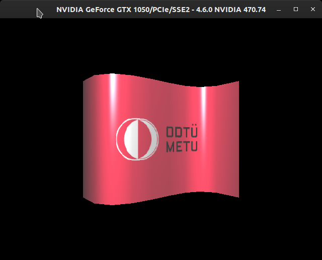
Normal Calculation

I committed major stupidity while implementing normal computation.

I used the method presented in the slides. It made use of partial derivatives to find two perpendicular vectors which yield the desired normal at any given point. That was not bad for high sample counts, and I gained experience. However, when the sample count is reduced, it created weird artifacts since the normal calculation does not consider the discretized version of the surface, it just computes normals for the underlying Bezier surface.

Here, you can see the artifacts created by faulty normal calculation:

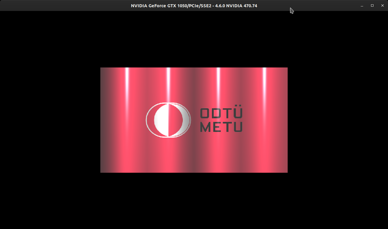
The funny thing is, this detail was already specified in the assignment document. But I skipped it while quickly reading through it. Instead of the previous method, we were advised to compute the normals by taking the average of the normals of neighboring triangles.

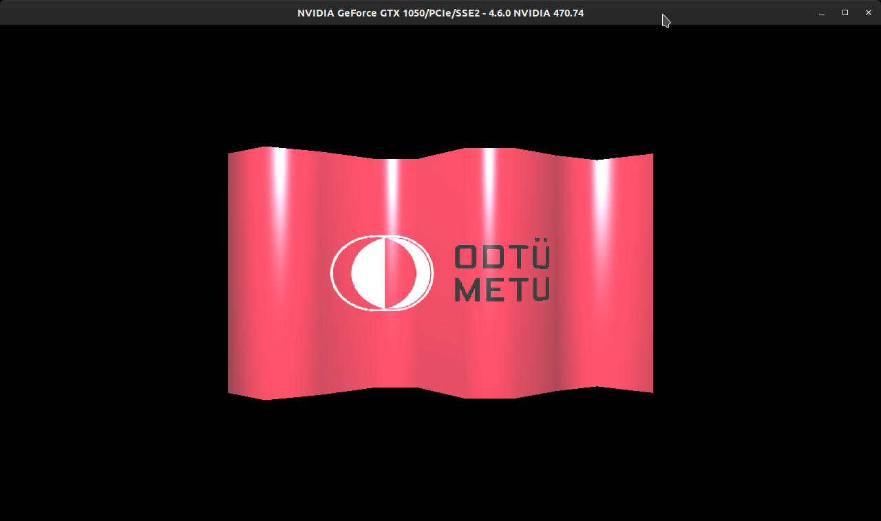
I implemented the new method, but some normals were not right. See the top side:

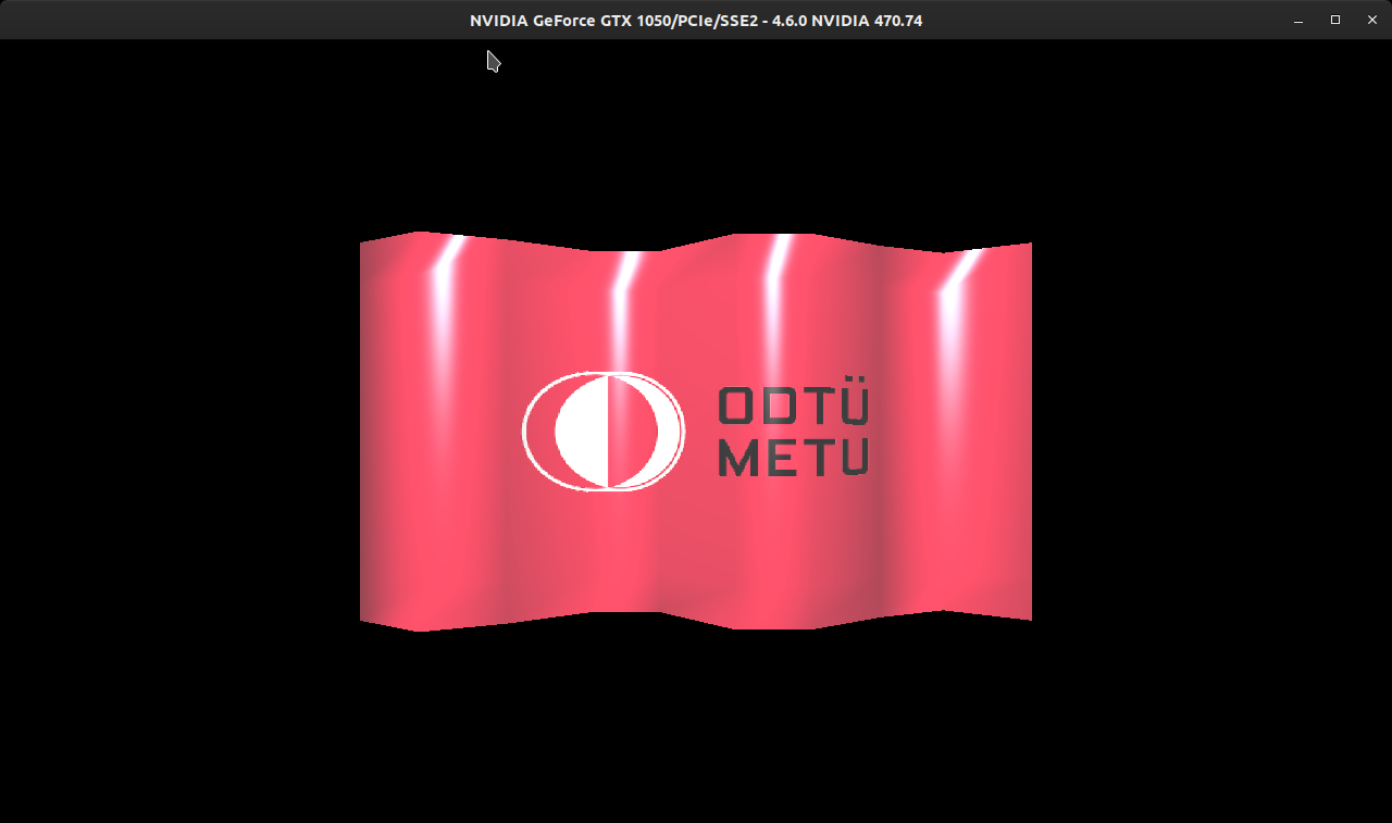
This happens because not all neighboring triangles have the same weight. In some triangles, the angle at the given vertex is large, whereas in others, it’s about the half.

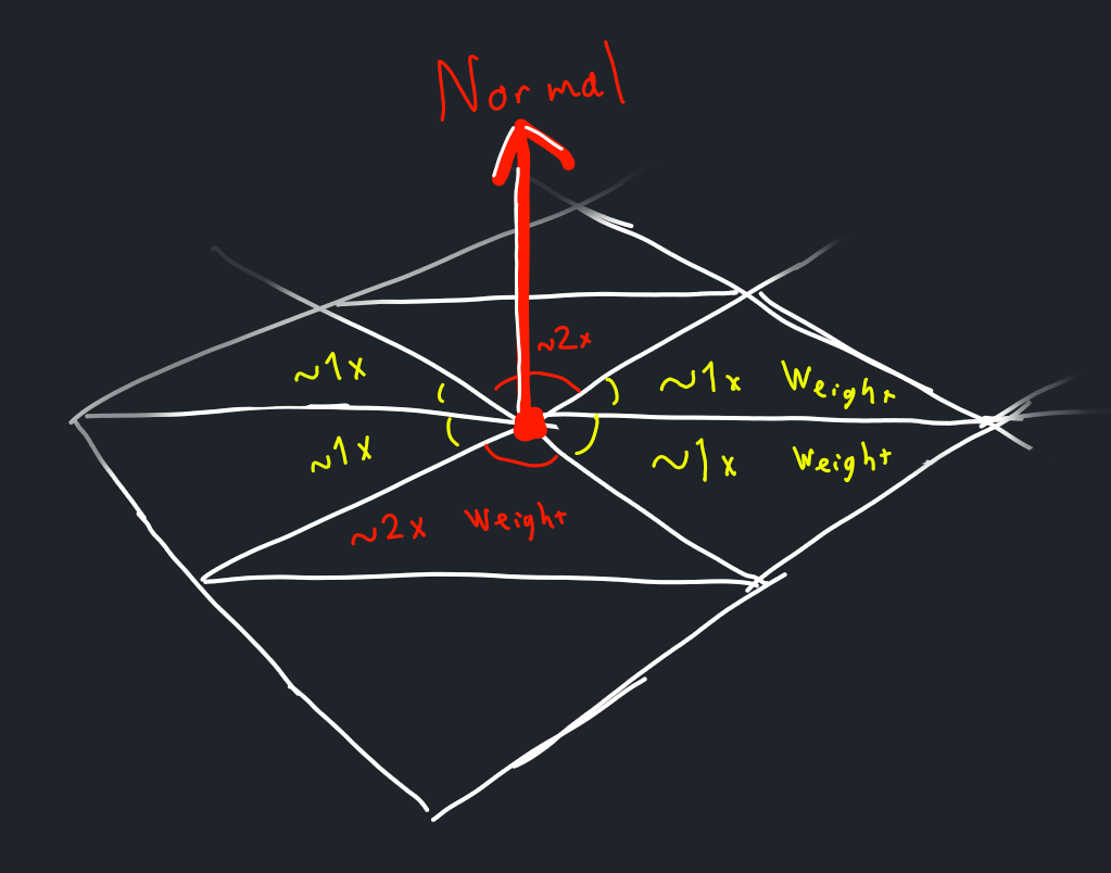
A rigorous solution would calculate the angle of each triangle at the given vertex and weigh their normals accordingly. But I decided to follow a simple heuristic to solve this problem. Note that in some cases, the vertex divides the neighboring rectangle in half. In these cases, I added the normals of the triangles that compose that rectangle once. In other cases where the vertex resides at the 90 degree angle, I added the normal of that triangle twice.

In the end, this method seemed to work well. Since this operation is performed at CPU (cannot access neighboring vertices in vertex shader), I tried to preserve as much computing power as possible.

Multiple Patches

A Bezier surface maps two parameters \(s \in [0, 1]\) and \(t \in [0, 1]\) to \(\mathbb{R}^3\). In order to sample from multiple patches, we need to devise a partial function.

Here’s an example. The following function \(F(s,t)\) maps \(s \in [0,2]\) and \(t \in [0,2]\) to a surface that is composed of 2x2 Bezier surfaces, named \(Q_1\) to \(Q_4\).

\[F(s,t) = \begin{cases} Q_1(s,t) & \text{ if } 0 \leq s < 1 \text{, } 0 \leq t < 1 \\ Q_2(s,t) & \text{ if } 1 \leq s < 2 \text{, } 0 \leq t < 1 \\ Q_3(s,t) & \text{ if } 0 \leq s < 1 \text{, } 1 \leq t < 2 \\ Q_4(s,t) & \text{ if } 1 \leq s < 2 \text{, } 1 \leq t < 2 \\ \end{cases}\]

With this approach, the implementation was fairly easy. However, making the surfaces move together was a challenge. To achieve this, I fine-tuned the parameters of sine wave functions that orchestrate the animation process.

Animation

We have been given lots of liberty in this regard. The only constraints are:

1. The animation must be smooth, no sudden jumps.
2. G1 continuity must be preserved.
   • The derivatives should match at the edges between the patches.
     • This is satisfied in Bezier curves when the control points corresponding to an end-point in both surfaces are colinear.
   • Intiutively, this means that hte surface of the flag must be smooth.

I collected some animations from online sources for reference. The most helpful one was the following:

If you focus on the top or bottom side, you will observe that it’s basically a sine wave function, shifting in space as time passes. However, if you just move the z-axis of control points with sine wave, you will find that there will be times when the whole flag becomes flat:

Unlike the first sample animation, this one doesn’t seem natural. The waves are not going towards the wind direction; they are just disappearing and appearing again.

At first I thought that achieving the exact same animation was impossible due to the limitations of Bezier curves. They are based on polynomials after all, they cannot simulate a sine wave with 100% accuracy, as they cannot create a circle. However, it should be possible to approximate.

At first, I thought that a patch should cover a single period of sine function. Because when the end points are at z = 0 and control points are at positive z and negative z respectively, we get a nice curve that looks like a sine wave. However, this approach was doomed from the start: it wasn’t possible to represent the curve when the sine wave is shifted.

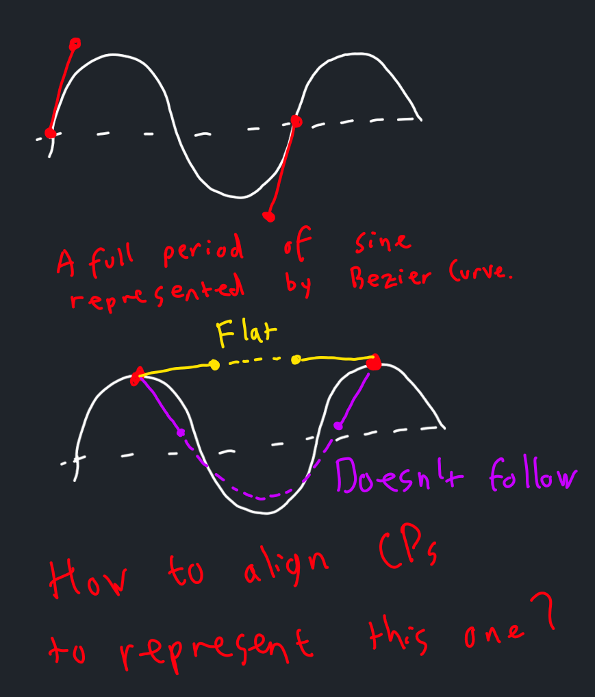
As a result, I decided that a patch should only cover half of the period. I thought about the initial case and the transient states as the sine wave slides.

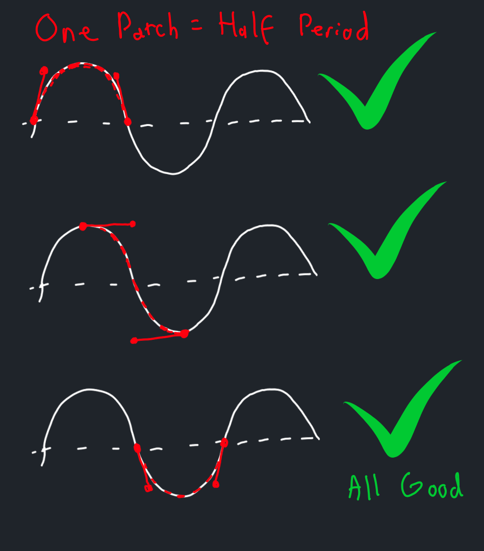
By carefully examining these cases closely, we can come up with a generalized rule for this animation. The details are given in the next drawing. Here we reason about the location of each control and end point in relation to others. T=0 means that the point is at the start of a period, and T=1 means the end of a period.

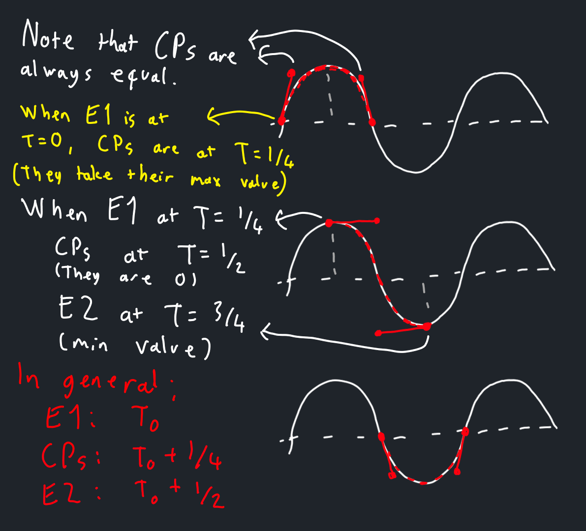
After adjusting the parameters in sine wave functions by trial and error, I was able to create a nice vertical wave animation. How the wave looks with 12 samples and 3 patches:

I was worried that the flag would look weird when there’s only one patch. But it ended up looking quite good, this one is with 12 samples and 1 patch:

Vertical Movement

The animation looks good, but all waves are completely vertical. There should be some movement in the horizontal direction as well.

If you refer back to the reference image I borrowed above, you will see that the sine waves get shifted as we go up and down the flag. This can be implemented simply by adding the y component of a point to its phase. In other words, if we are given the animation function \(sin(2 \pi t)\), we can turn it to \(sin(2 \pi (t + y))\) so that some points get “delayed” based on their y coordinate. Of course we need to adjust the formula so that the G1 continuity is preserved and the animation looks good, but this is the basic idea and I won’t bore you with details.

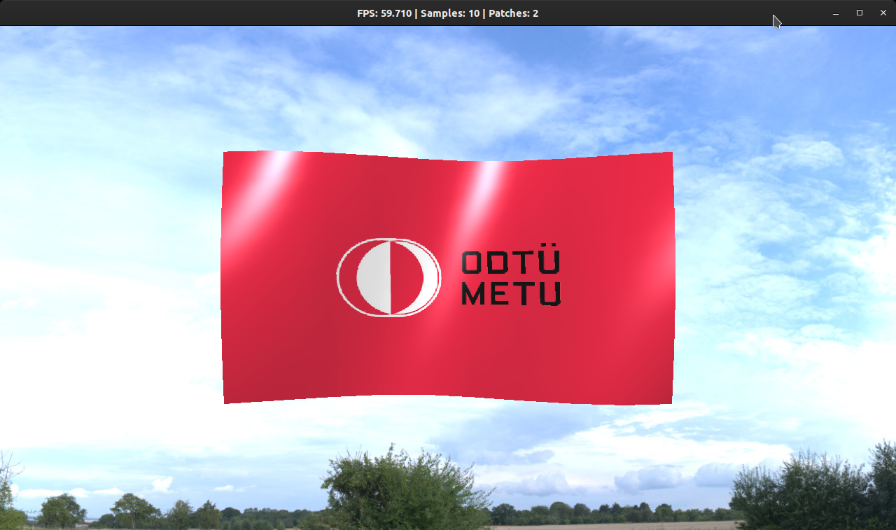
Here’s the state of the flag after this update. The animation looks quite close to my reference gif image now.

By the way, I added a plane with a texture to the background for the sky. Moreover, I refactored the code a little bit so that both the flag and the sky uses common code for reading textures, using shaders etc.

Improving the Animation

At the current stage, only the z coordinates of control points are animated. Obviously, that’s not how a real flag behaves in real life, so there’s room for improvement.

We need to be careful about the G0 and G1 continuity while moving the end-points. To preserve these, I moved the corresponding control points each time I moved an end-point, and the neighboring end-points of surfaces have the same motion. As we will see, I almost exclusively used trigonometric functions (namely sine) while moving the points. Consequently, it wasn’t hard to maintain the smoothness of the animation.

The first kind of movement I wanted to implement was shifting the center of the flag along the x axis. (Note that the camera is looking down in -Z direction with +Y up.) First I mapped y coordinates of the flag to \([0, 1]\) range. After that, I fed the result of this mapping to \(f(x) = sin(\pi x)\). Now the sides are mapped to 0 and the center of the flag is mapped to 1 with a nice arching shape inbetween. Excellent.

After that, I wanted to alter the y component of the control points. Naturally, a flag will fall down as it gets farther away from the pole. To emulate this effect, I simply made the y component decrease linearly as the point moves towards the right side.

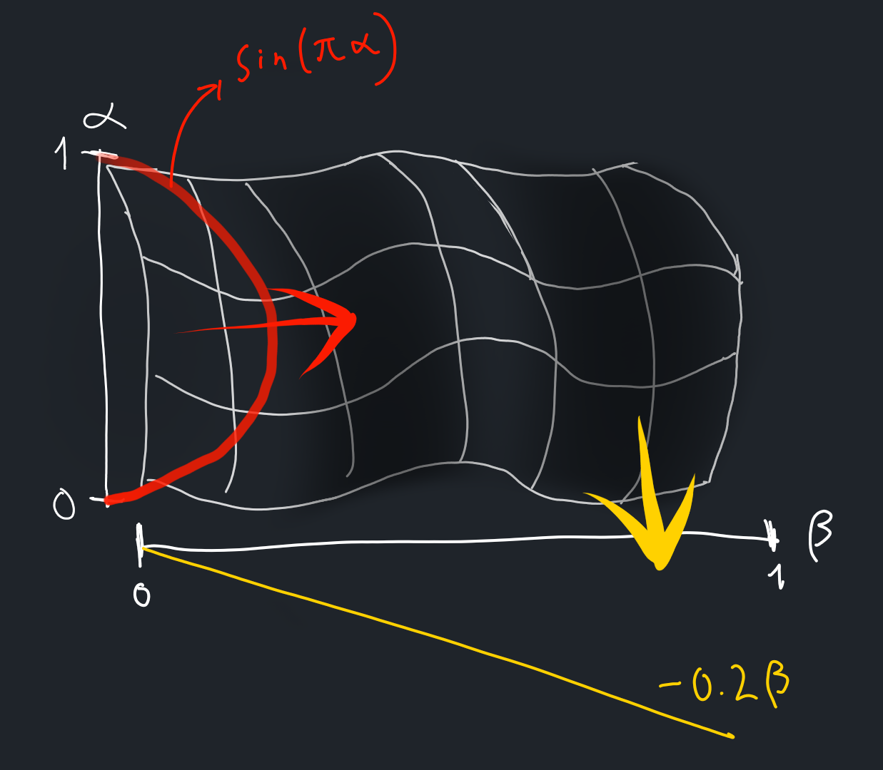
Now, we have these transformations. How do we actually animate and combine them? In my opinion, these should not be simultaneous animations but complementary ones, because the first transformation happens under strong wind, whereas the second one happens in the opposite case.

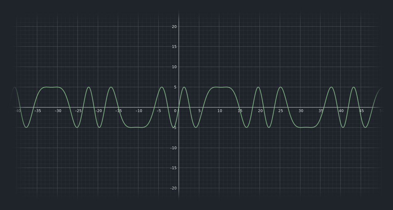
To make the animation more lively I decided to alter the speed of animation at various intervals. Then, we can use the speed parameter to figure out the influence of the aforementioned transformations. To this end, I used (guess what) sine functions. We want the speed to change at various intervals, but unlike a regular sine function, we don’t want it to go with a predictable pattern.

To add some chaos and randomness, I used the following as speed function: \(speed(t) = sin(8.0 sin(0.15 x)) + 2.0f\)

Its graph looks like this (+2.0f is ignored and scaled along x axis by 5 for better viewing experience):

Combining it all together with transparent texture support, alpha blending, and a new flag texture yields the following results. 20 samples and 3 patches were used:

Apparently this flag is Railroad Flag from Fallout 4, borrowed from Fallout Wiki. Never played that game, but I found its flag while searching for a flag texture with alpha channel.

Normal Maps

I implemented support for normal maps, following the guidance of LearnOpenGL website.

We define the base geometry of an object using vertices and triangles, but the small imperfections on the surface of an object will affect the lighting as well. Normal maps attempt to emulate this by encoding the surface normals of a texture into an RGB image. In the shader, these colors are converted into normal vectors and used in lighting computations. Normal maps allow us to easily increase the realism without causing significant performance penalty.

For example, the following flag features a normal map:

And here’s the video I submitted to the flag competition:

Failed Experimentations

I tried to combine multiple waves of different frequencies and sizes, but this change almost always broke the G1 continuity. I believe it’s possible to do this but the time wasn’t enough.

Performance

Even though I avoided premature optimization as much as possible, I preferred to go with the approaches that I deemed to be performant without sacrificing code readability and maintainability.

My GPU is NVIDIA GeForce GTX 1050/PCIe/SSE2 with driver version 470.74. I have an Intel i7-7700HQ (8) @ 3.800GHz CPU with 16 GB of RAM. While testing the program during development, I didn’t run into any performance problems. I usually tested with about 20 samples and 3-4 patches. The program was able to maintain a pretty much consistent 60 FPS. Apparently GLFW caps the FPS at 60 because I am not able to reach a higher value even with an empty window.

When I reach 50+ samples and 20+ patches, I start to run into some performance complications, albeit weird ones. After setting the sample and patch count to high numbers, the program runs for a while at 60 FPS, and then drop to ~20 FPS momentarily, only to rise up to 60 FPS again. These FPS dips happen periodically as long as the sample and patch count is kept high.

I couldn’t find any reason for this. Since there were no FPS constraints on this assignments and the inek computers are much better than mine, I decided to invest my limited time to other parts, such as animation.

Conclusion

I really enjoyed this homework. Genuinely, it was one of the best assignments I got in my undergraduate years. It gave us lots of freedom while guiding us through the boring parts. Since there were not many constraints on animation, I had to figure it out by myself and learned a lot along the way. The only thing I regret is starting this homework late. I wish I had more time to work on this.

Thanks to AmbientCG and PolyHaven for textures.